Signal Processing Window

The signal processing window is the central part of the Signal Processing Task. It is here that all signal processing is configure and also here the actual processing is executed.

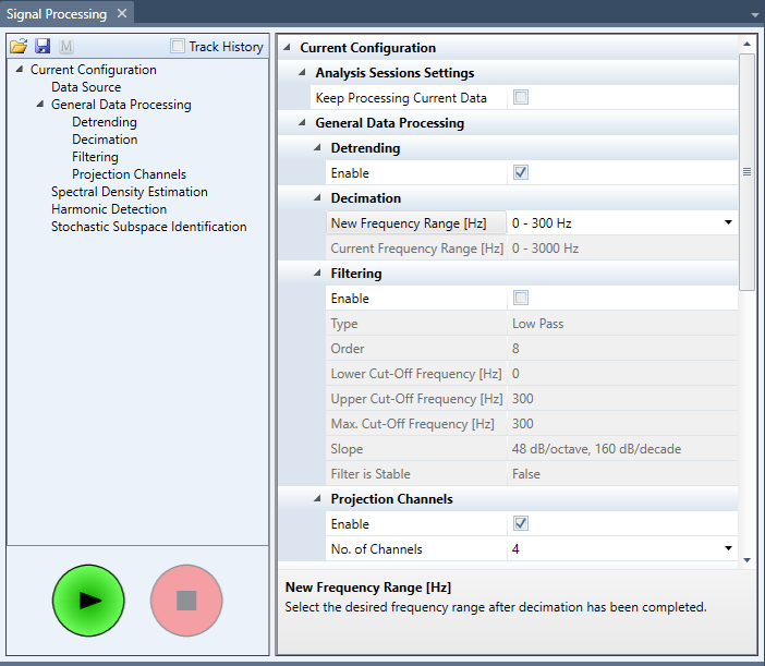
In the top left part of the window there is a three view that you can use to navigate through the different settings. Below there are two buttons. The green is the Start Signal Processing button that you hit when the settings are in order. If you need to abort the processing use the red button. While the processing is going on messages will be written to the Output window informing about the current status of the processing.

To the right there is a grid view listing all the different settings that you can manipulate. Below a full description of these settings is given.

Current Configuration - Data Source

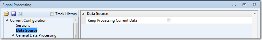
ARTeMIS Modal is using the compound file that stores the raw measurements and the processed measurements in two different sections. When the Keep Processing Current Data check box is disabled, like in the above picture, the signal processing start with a copying of the raw measurements to the processed measurements section. In this way all previous signal processing is forgotten. Disabling the Keep Processing Current Data is the default setting when starting working with the data first time and can later on be disabled in order to re-start the processing again with a fresh copy of the measurements. After first run the setting automatically change to enabled.

General Data Processing - Detrending

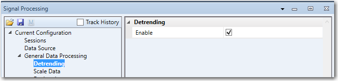
Detrending means removal of the mean value as well as any linear trend that may be in the measurements. A linear trend could be caused by e.g. drift and it is removed by fitting a first order polynomial to each of the measurement channels and then subtracting it afterwards. By default linear trends should be removed since they can disturb the signal processing and modal analysis. This type of processing is irreversible and will modify the measurements. If you later wish to change this setting you should always start by reloading a fresh copy of the measurements by un checking Keep Processing Current Data.

General Data Processing - Overall

In case a Master Session is defined and the currently active session is not the Master, then the General Data Processing is disabled. In any other case, it is Enabled.
As mentioned above, since the Damage Detection Plug-In can obtain the correct results only if the same GDP settings are used in all sessions, if changes are required then the user must activate the Master Session and re do the Signal Processing in all sessions.

General Data Processing - Scale Data

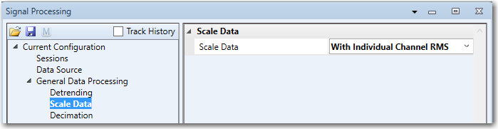
Scaling of the data is to enhance the accuracy of the analysis in case of the following:
1. There is a big difference of amplitudes in the different channels. ->Individual Channel RMS Scaling
2. The measurements are in general e.g. very small or very big -> With Max Channel RMS

General Data Processing - Decimation

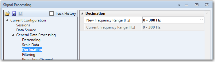
The purpose of decimation is to reduce the frequency range to the frequency range of interest. For instance, if a signal has been sampled at 200 Hz, i.e. 200 samples
per second, then the Nyquist frequency is 100 Hz and the Spectral Density Estimates will be defined in the interval from 0 - 100 Hz. Now, if only you are interested
in the modal properties lower than 10 Hz you should decimate the signal 10 times.

If you want to work in the frequency domain it is desirable to decimate to zoom to the range of interest. If you are working with parametric models in the time domain,
you should decimate in order to introduce poles only in the frequency range of interest.

The decimation is basically a process where some samples are discarded and some samples are kept. However, in order to prevent aliasing the signal is first low-pass filtered
and then the excessive samples are discarded. If the signal is decimated 2 times then every 2nd sample is kept and the rest is discarded. If the signal is decimated
3 times every 3rd sample is kept the rest is discarded, etc.

Now, since the anti-aliasing filter is active into the frequency range of the decimated signal, you should only use the modal results in the frequency range from 0 to 80
% of the new Nyquist frequency. The applied anti-aliasing filter is an 8th order Chebyshev Type 1 low-pass filter.

This type of processing is irreversible and will modify the measurements. If you later wish to change this setting you should always start by reloading a fresh copy of the measurements by un checking Keep Processing Current Data.

In the drop down list you can see the available frequency ranges depending on the level of decimation. If the Keep Processing Current Data is enabled the possible frequency range will smaller and smaller for every time you decimate the data.

General Data Processing - Filtering

Filtering is used to shape the signal in the frequency domain. A typical reason for filtering could e.g. be to high-pass filter the signal to get rid of a slowly varying
zero-offset of the signal, or to band-pass filter the signal to reduce the necessary parametric model order for cases with high modal density.

You have the possibility to apply one of the following types of filters: low-pass, high-pass, band-pass and band-stop. In each case the filter is of the Butterworth
type and you can select filter orders between 1 and 50. The Butterworth filter is a good all-round filter that is simple to use. At the specified cut-off frequencies
it attenuates 3 dB.

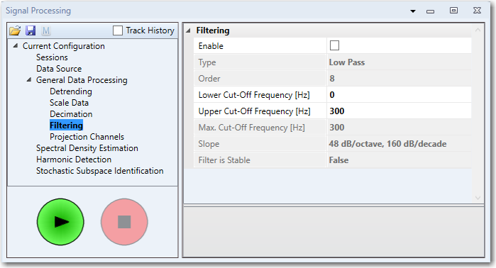
As seen is Filtering by default disabled. If you do not want to specify any filter just keep the default settings. To enable filtering check the Enable box.

The default filter type to appear is an 8th order low-pass filter which is a reasonable order to start from. You can then select different types of filters from the Type
drop down list and different order from the Order edit field. The order depended slope of the filter is presented both in Slope per octave and Slope per decade.

If the filter is unrealizable you will not be able to start the signal processing on the green button. The most common reason for a filter to be unrealizable is that the filter is unstable.
To reduce the risk of a filter becoming unstable, choose a lower model order or move the cut-off frequency further away from the frequency boundaries, i.e. towards the
middle of the frequency band from zero to the Nyquist frequency.

General Data Processing - Projection Channels

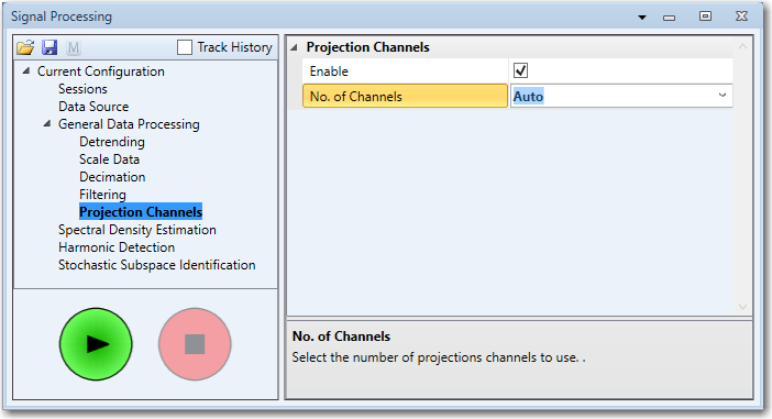
To avoid too much redundant cross information when estimating spectral densities and the state space models in the Stochastic Subspace Identification techniques you should always activate Projection Channels. By default this option is enabled and set to Auto which indicate that the software by itself will try figure out how many projection channels to use for the specific data.

Alternatively, you can also run the processing without enabling Projection Channels and then study the Singular Value Decomposition in the Processed Data window. Count how many singular value lines you need in order to reach the first one that is reasonably flat in the frequency range you like to study. The number of lines you counted is a very good number to select in the No. of Channels drop down list above.

Technically, what is selected is actually the column space to make use of in the estimation of spectral density matrices. In case of the Common SSI Input Matrix estimation in the Stochastic Subspace Identification techniques it corresponds to the selection of the row space to project the measurements onto.

The selection of the projection channels is done automatically. The first columns chosen are the reference channels if they are available. The rest of the columns are the ones that on average correlates the least with the reference channels. This is done to maximize the amount of independent information.

Spectral Density Estimation

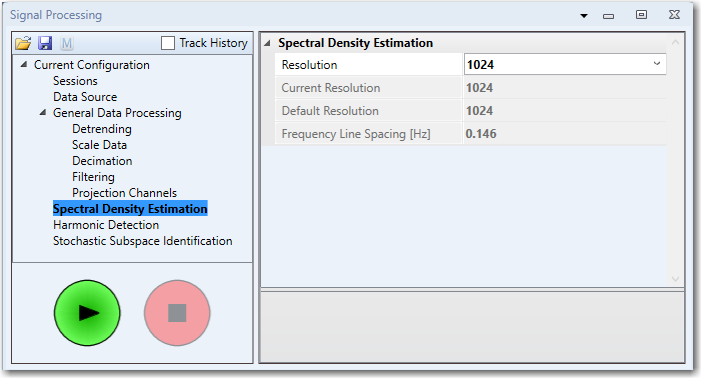
In the Spectral Density Estimation section you specify the frequency Resolution of the spectral density diagrams, i.e. how many discrete equally spaced frequency lines in a range between zero (DC) frequency and
the Nyquist frequency. Below the drop down list you can see what current resolution has been applied as well as the default one. Finally, it can be seen what Frequency Line Spacing in Hz the currently selected resolution is causing.

Note: The estimation of spectral densities is always performed with 66% overlap and using a Hanning window.

Harmonic Detection

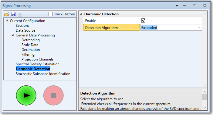
Since not all signals have deterministic signal creating "harmonic peaks" in the spectral densities the Harmonic Detection is not enabled by default. To enable it simply check the Enable check box. This option is only available when the Projection Channels are enabled.

Two options for harmonic detection are available when the check box has been enabled, which are an Extended Kurtosis Check and a Fast Check. When the first option is chosen the Kurtosis is estimated for every single frequency line (0 - Nyquist). Since this option is a time-consuming process, another option, the Fast Check, is available. By this method the singular value curves are all searched for possible harmonics before the kurtosis is estimated for the identified candidates. In order to have enough singular value curves to identify the harmonics from at least 4 - 6 projection channels should be chosen.

Stochastic Subspace Identification

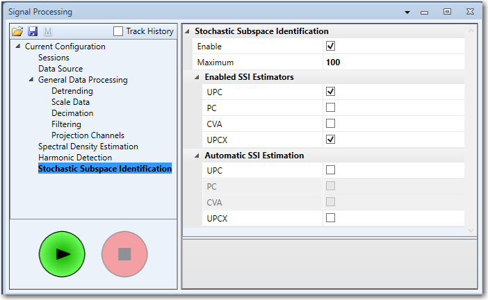
The computational part of the Stochastic Subspace Identification (SSI) that is most time consuming is the estimation of the Common SSI Matrices (one per Test Setup) that is used by all the different SSI techniques.

The initialization of the Common SSI Input Matrix Estimation is something that you cannot really do before you have looked at the data or processed what is needed to inspect the spectral densities in the View Processed Data window. The reason is that you need to have an idea of how many modes that are present in the data. In order to overcome this problem usually a reasonable high dimension like 80-100 is used. If there are many modes this might not be enough, but for most cases it will be.

The modes that are estimated using the Stochastic Subspace Identification techniques can be grouped into the following types: Structural modes, harmonics, and noise modes.

Usually, it is the structural modes that we are interested in since these describe the dynamics of the structure we are analyzing. Besides, in these modes there will also be harmonics in the data as soon as there are rotating parts in the structure or in the excitation. Finally, there will always be noise modes or computational modes present. They are not always easy to see in a spectral density plot because of their tendency of being highly damped. However, you will always have computational modes arising e.g. from the anti-aliasing filter. Computational modes also appear if your system is not completely linear, or if the excitation is far from being a
realization of a shaped Gaussian white noise, or if in other ways the assumption for using the estimation techniques are not met. The computational modes are then added by the estimation algorithm to take account of the discrepancies.

It is usually a very good idea to inspect the Singular Value Decomposition of the Spectral Density Matrices because this very elegantly reveals the structural modes, the harmonics and any close spaced modes. By counting the structural modes and the harmonics you will be well prepared for making the initialization of the Common SSI Input Matrix Estimation.

Automatic SSI Estimation

In case the SSI is enabled, then the ARTeMIS Modal allows that the SSI Estimation is done automatically during the Signal Processing, without having to go to the Modal Estimation Window and perform the estimation on each of the SSI estimators separately. This can speed up the analysis process, as you may immediately retrieve all of the SSI Modes. In case of multiple test setups, the UPC Merged is also available in the list.

Signal Processing Toolbar - Signal Processing Journal

Starting from version 3.0 the Signal Processing toolbar is introduced

The main purpose of this toolbar is the Signal Processing Journal Management. In case the Track History option is checked, each of the Signal Processing Settings is stored in a list in a consecutive order. The Signal Processing Journal can be used in case you need to apply the same processing settings on the same or a similar project and instead of configuring the settings each time you can simply load the settings which will be automatically applied upon loading.

The Save button is used to export the Signal Processing Journal to an xml file.

The Open button is used to open an existing Signal Processing Journal File (.xml) and apply the Signal Processing to the current project.

Signal Processing Toolbar - Switch to Master Session

The button is used to quickly switch to the Master Session, so that new Signal Processing can be applied to the sessions. The button is enabled only if a Master Session is defined and the currently Active Session is not the Master Session.